In recent years, Cloud Model 1 (CM1; http://www2.mmm.ucar.edu/people/bryan/cm1/) has become a very popular tool for performing idealized studies of atmospheric phenomena. There exists very little support for computing trajectories using CM1 output, which are usually necessary to understand the processes of the atmospheric phenomena of interest. Natively, CM1 only supports 'online' forward trajectories in 2D simulations and in 3D simulation without terrain. I wrote this script because there are no adequate tools available to compute highly customizable 'offline' trajectories in simulations with terrain. This script is intended to be easily customizable. 'trajectories_CM1.ipynb' initializes and computes parcel trajectories and 'trajectory_plot.ipynb' produces a sample plot of the parcels' trajectories.
As of 3/21/2019 there are two versions of the code:
- trajectories_CM1.ipynb simply uses first order Runge-Kutta (Euler's method)
- trajectories_CM1_2nd_order.ipynb uses a second-order semi-implicit discretization in space and time. The discretized equations are presented in section 2.1 of Miltenberger et al. 2013 (https://www.geosci-model-dev.net/6/1989/2013/gmd-6-1989-2013.pdf) and is the generally accepted method for computing trajectories.
Notes:
- Can compute backward or forward trajectories (Default is backward, but can be forward with simple changes to "Calculate Trajectories" block)
- Written to work with 3D model output (can be modified to work with 2D output)
- Will work with or without terrain
- Will work with staggered or unstaggered u, v, and w fields
- Initial location, number, and density of parcels can be easily specified in "Initialize Parcels" block
- Uses xarray and Dask to distribute memory and calculation across multiple processors
- With modifications, can be used with WRF output (several others have already done so)
- Comments that say "set by user" are specific to model output and desired trajectories
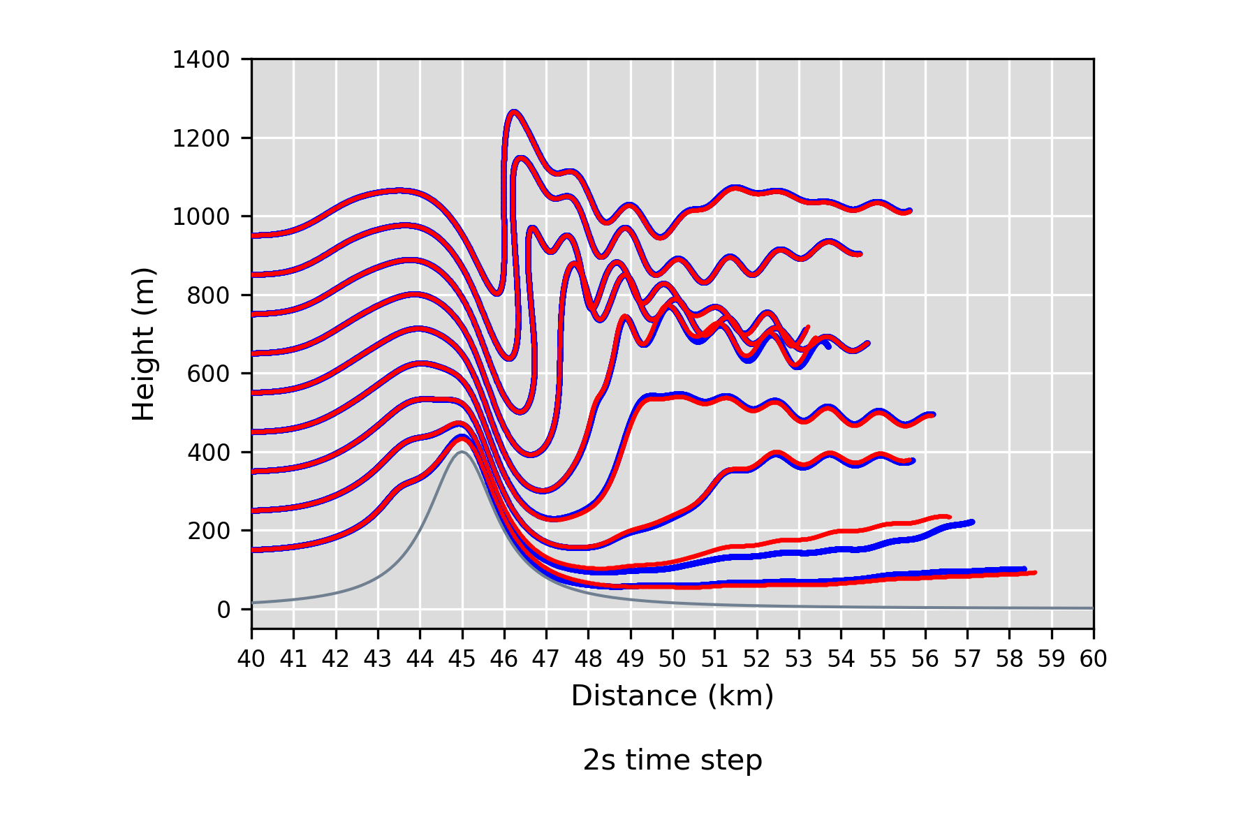
Trajectories computed with this code have been verified against trajectories computed within CM1 model integration (i.e., "online" trajectories). Verification was performed using a simple 2D mountain wave simulation. Trajectories in blue were computed "offline" using the code here (trajectories_CM1.ipynb), while trajectories in red were computed "online", within the model integration. The "offline" (blue) trajectories very closely match the "online" (red) in this nonlinear, turbulent flow, indicating that trajectories_CM1.ipynb is correctly computing "offline" trajectories.
Questions? Email me at [email protected]
