Machine-Learning-Predictive-Modelling

List of various Machine Learning algorithms used in projects.

1) Predicting Car Prices using k nearest neighbors algorithm

The dataset used was found here.

The goal of the project was to determine which were the best features to use to predict a car's price, and then to see how accurate the predictions were using those models.

Data Processing

The dataset went through an initial round of processing that included:

• adding column names
• changing the type of a column where necessary
• changing column values where necessary
• removing or filling missing values
• dropping unnecessary columns
• normalizing of numeric columns

Univariate and Multivariate Modelling

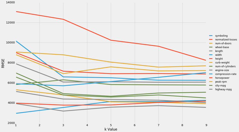
Univariate Modelling was initially used to determine what the best features for modelling might be. This was done varying the k value (n_neighbors) hyperparameter in the KNeighborsRegressor function.

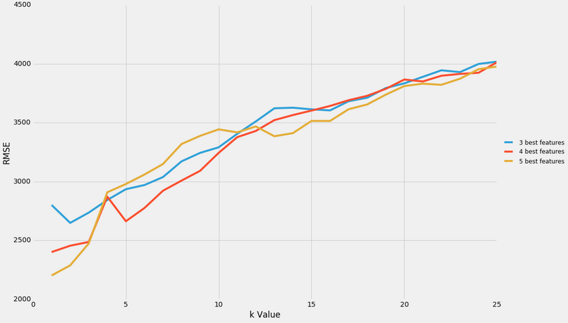
Thereafter, the best features were isolated, and multivariate modelling was performed using the 3 best, 4 best, and 5 best features, with the k value parameter varied from 1-25.

It was determined that:

1. Predictive modelling should be performed using the 4 or 5 best features (the 5 best being, in order of best to worst, ['engine-size', 'width', 'horsepower', 'highway-mpg', 'curb-weight'].
2. A k-value of 3 or less should be used to minimize the root mean squared error value.

2) Predicting House Prices using Linear Regression

The dataset can be found here. This dataset was originally compiled by Dean De Cock for the primary purpose of having a high quality dataset for regression.

A pipeline of functions was set up to allow us to quickly iterate on different models, consisting of the transform_features, select_features, and train_and_test functions.

Feature Engineering, Feature Selection, and K-Fold cross validation were used on the original data-set to predict the price of houses in the city of Ames, Iowa, United States.

Feature Engineering

• Any column with more than 15% missing values was dropped.
• For text columns in particular, we dropped cols with any missing values at all.
• For numeric columns, we imputed missing values as the average of that column.
• Created new features based on existing columns, such as no. of years until a house was sold.
• Dropped columns that weren't useful, or which leaked data on the sale.

Feature Selection

• Identified numeric columns that correlated strongly with target columns, and selected those with strong correlations (> 0.4)
• Converted any remaining nominal features to categorical type.
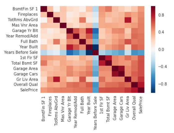
• Generated Heatmap to identify collinearity between columns.

K-Fold Cross Validation

The train_and_test function was modified to accept a parameter k which controlled the type of cross validation that occured:

1. When k = 0 , holdout validation was be performed, which is what the function did by default.
2. When k = 1, simple cross validation (first time with train and test sets, second time with them swapped) was performed, and then the avg rmse was returned.
3. When k > 1, k-fold cross validation was performed using k number of folds.

3) Linear Regression - Stock Market Prediction (S&P500 Index)

In this project, we worked with the sphist.txt file (provided in this repository) containing index prices.

Overview

Each row in the file contains a daily record of the price of the S&P500 Index from 1950 to 2015. The model was be trained on data from 1950-2012, and then used to make predictions for 2013-2015. Feature engineering was carefully applied to reflect that stock market prices were not independent occurrences (because they're influenced by the stock prices from the recent days), and new features were added that accounted for this.

In the end, after some experimentation, we managed to produce a predictive model, using linear regression, with a relatively low RMSE of 22.18.

Future Improvements

Some future improvements could be:

1. Including even more indicators, like day of the week, no. of holidays in the previous month, etc.
2. Making Predictions only up to a week, or even only a day in advance.
   • For instance, data from 2014-05-20 and earlier could be used to predict prices on 2014-05-21.
   • This more closely resembles how people actually do stock market prediction using algorithms.
3. Using different algorithms, like a random forest, and seeing if they perform better.
4. Inclusion of data external to the provided dataset. For instance, we could look at things like:
   • The weather in cities where most trading happens
   • The amount of twitter activity surrounding a certain stock
   • Sentiment Analysis of a certain stock, using for instance Twitter data.
5. Making the system real-time by writing an automated script to download the latest data when the market closes, and then using that to make predictions for the next day.

4) Decision Tree and Random Forest Regression - Predicting Bike Rentals

Overview

Information on Bike Rentals from a dataset found here were analyzed to predict the number of bikes that would be rented in each hour.

Various predictive algorithms were used, such as Linear Regression, Decision Tree Regression, and Random Forest Regression. In the end, we discovered that the Random Forest Regressor algorithm unsurprisingly created the model with the best predictive accuracy. Linear Regression on the other hand did not fare well because it wasn't able to accurately model the few non-linear features that were in the dataset.

5) Classifying Hand-written Numbers using Deep Neural Networks

Overview

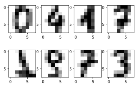
The load_digits() function from the scikit-learn library (accessible within the namespace of sklearn.datasets) was used to retrieve a copy of hand-written digits from the UCI machine learning repository.

After being retrieved, the data was then reshaped, and some of it was visualized to understand what we were working with.

Thereafter, Machine Learning algorithms were used to attempt to classify the digits above.

1. K Nearest Neighbor algorithm was initially used to get a benchmark value for accuracy (measured using simple accuracy, i.e. correct predictions/total predictions)
   • Unlike the linear and logistic regression models, the K-nearest neighbours algorithm makes no assumption about linearity between features and the output labels. This allows it to capture nonlinearity in the data.
2. Afterwards, deep neural networks were used.
   • Deep learning tends to be effective in image classification because of the fact that its models can learn hierarchical representations. An effective deep learning model learns intermediate representations at each layer in the model, and then uses them in the prediction process. Each successive layer uses weights from previous layers to try and learn more complex representations.
   • Various parameters, like the number of neurons, and number of hidden layers were tuned to see how it would improve accuracy.
   • As the no. of hidden layers increased, we increased the amount of folds used in k-fold cross validation to minimize over-fitting. This was to get around the fact that increasing the number of hidden layers generally results in an increase in the model's overfitting.
   • Using 3 hidden layers with over 250 neurons resulted in very high accuracy rates of over 96%, which is cohesive with research literature about using deep neural networks for computer "vision", such as the digits classification we attempted here.