Map structures for vectored maps to use with ggplot2

[dicook]

I find myself often re-doing the same code to extract data from a map repository, extract the polygons, and identifiers, in order to make chloropleth maps, or map backgrounds for spatial data. For example:

#### Set up map - yes, pbly should be recoded with purrr
world <- getMap(resolution = "low")
extractPolys <- function(p) {
  polys <- NULL
  for (i in 1:length(p)) {
    for (j in 1:length(p[[i]]@Polygons)) {
      x <- p[[i]]@Polygons[[j]]@coords
      polys$lon <- c(polys$lon, x[,1])
      polys$lat <- c(polys$lat, x[,2])
      polys$ID <- c(polys$ID, rep(p[[i]]@ID, nrow(x)))
      polys$region <- c(polys$region, rep(paste(p[[i]]@ID, j, sep="_"), nrow(x)))
      polys$order <- c(polys$order, 1:nrow(x))
    }
  }
  return(data.frame(polys))
}
polys <- extractPolys(world@polygons)

#### Map theme
theme_map <- theme_bw()
theme_map$line <- element_blank()
theme_map$strip.text <- element_blank()
theme_map$axis.text <- element_blank()
theme_map$plot.title <- element_blank()
theme_map$axis.title <- element_blank()
theme_map$panel.border <- element_rect(colour = "grey90", size=1, fill=NA)

#### Plot 
qplot(lon, lat, data=polys, group=region, geom="path") + 
  theme_map + coord_equal()

#### Merge data with map
#### Match country names to map names
cntrynames <- unique(datraw$country)
polynames <- unique(polys$ID)
setdiff(cntrynames, polynames)

#### Tabulate the countributing countries
cntry_count <- datraw %>% group_by(country) %>% tally()

#### Join to map
polys_cntry <- merge(polys, cntry_count, by.x="ID", by.y="country", all.x=TRUE)
polys_cntry <- polys_cntry %>% arrange(region, order)
ggplot(data=polys_cntry, aes(x=lon, y=lat)) + 
  geom_polygon(aes(group=region, fill=n), color="grey90", size=0.1) + 
  scale_fill_gradient("", low="#e0f3db", high="#43a2ca", na.value="white") + 
  scale_x_continuous(expand=c(0,0)) + scale_y_continuous(expand=c(0,0)) +
  coord_equal() + theme_map 

This is the code that I put together to look at the R contributor survey. I wonder if it would be a good idea to have this packaged for more generally working with spatial data.

[jonocarroll]

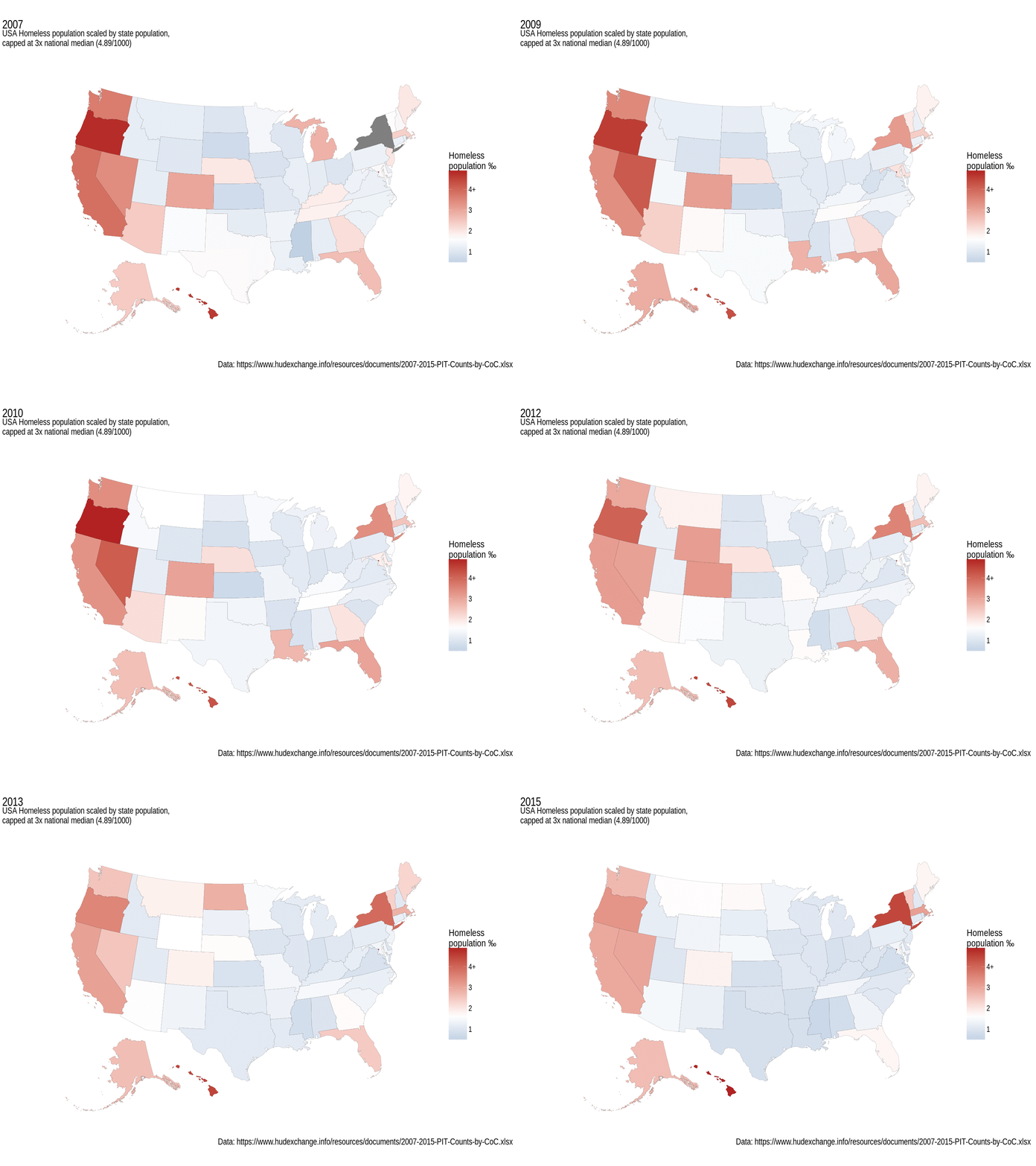
This is the other half of one of my ideas (though I limited mine to Australia); some good progress has been made in doing this for the USA so that now it's as simple as

library(albersusa) ## devtools::install_github("hrbrmstr/albersusa")
us <- usa_composite()
plot(us)

That package includes various regional breakdowns and applicable projection transformations.

I used this in a recent analysis, myself. The entire processing script (obtain data, process, generate output, save) is a mere 100 lines, including blanks.

I was hoping we could put together an Australian version, where the replicated data sets were easily available as aus@data. I repeated the above graph/analysis for Australia (blog post impending) and had to go through the same hassles as you describe to get to this point.

The map theme is covered by ggthemes::theme_map() .

Extending these to a global ensemble would be an interesting task.

[dicook]

Yes, exactly. But we’d like the rest of the world to be represented too.

On Apr 12, 2016, at 8:22 AM, Jonathan Carroll [email protected] wrote:

This is the other half of one of my ideas (though I limited mine to Australia); some good progress has been made in doing this for the USA so that now it's as simple as

library(albersusa) ## devtools::install_github("hrbrmstr/albersusa")
us <- usa_composite()
plot(us)

That package includes various regional breakdowns and applicable projection transformations.

I used this in a recent analysis, myself. The entire processing script (obtain data, process, generate output, save) is a mere 100 lines, including blanks.

I was hoping we could put together an Australian version, where the replicated data sets were easily available as aus@data. I repeated the above graph/analysis for Australia (blog post impending) and had to go through the same hassles as you describe to get to this point.

The map theme is covered by ggthemes::theme_map() .

Extending these to a global ensemble would be an interesting task.

—
You are receiving this because you authored the thread.
Reply to this email directly or view it on GitHub

---

Di Cook
[email protected]

[jonocarroll]

Yes, I'd be interested in that. Would hopefully be fairly streamlined if we took the purrr route. I was aiming for a more specific regional breakdown, which requires domain knowledge of each country, but at the country level most of your code should be portable to a function (possibly with a country subset argument), is it not?

[cpsievert]

It looks like ggplot2::fortify has a method for objects of class "SpatialPolygonsDataFrame":

class(world <- getMap(resolution = "low"))
# [1] "SpatialPolygonsDataFrame"
# attr(,"package")
# [1] "sp"
dat <- fortify(world)
qplot(long, lat, data=dat, group=group, geom="path") + 
  theme_map + coord_equal()

Are other types of geographic data structures that could use a fortify() method?

[jonocarroll]

I believe ggplot2::fortify is moving towards being deprecated in favor of broom::tidy.

Rather than using this function, I now recomend using the \pkg{broom}
package, which implements a much wider range of methods. \code{fortify}
may be deprecated in the future.

Though at the moment they're almost functionally equivalent.